EuroSAT Satellite Image Classifier
Fine-tune a CNN on EuroSAT Images
An implementation of a deep learning approach for land use classification from satellite imagery, aiming to reproduce the standard transfer-learning approach while building a foundation for further sensor modeling work. Built on a PyTorch ResNet18 backbone and trained on the EuroSAT Sentinel-2 dataset. The training pipeline was implemented independently to gain a deeper working understanding of the full workflow.
Dataset
I used the EuroSAT Sentinel-2 dataset12 of satellite images.
Dataset parameters:
- 27,000 images
- 10 classes
- RGB subset
- not the full 13 band Sentinel-2
- Images are 64x64 resolution
Approach
Data cleaning
I did the following cleaning items
- resize all images to 224 x 224
- ResNet18 expects all images to be 224 x 224
- randomly flip images vertically and horizontally
- Done to increase variety in the training sample.
- normalized images
- standardized to ResNet18’s RGB center and spread as defined by ImageNet. Using the center and spread expected by ResNet18 allows the model to reap the benefit of using pretrained weights.
- 70/15/15 split for training, validation, testing
Training
I used a transfer learning approach of ‘freezing and fine tuning’ a pre-existing model3.
- 8 epochs
- Freezing section: 3 epochs with a frozen backbone
- just trained the new 10 classes
- did not update the ResNet18 model
- Fine tuning section: last 5 unfrozen backbone
- Freezing section: 3 epochs with a frozen backbone
Results
- Test accuracy: 97.63% - within the range of the published benchmark for the EuroSAT dataset
- Test loss: 0.07
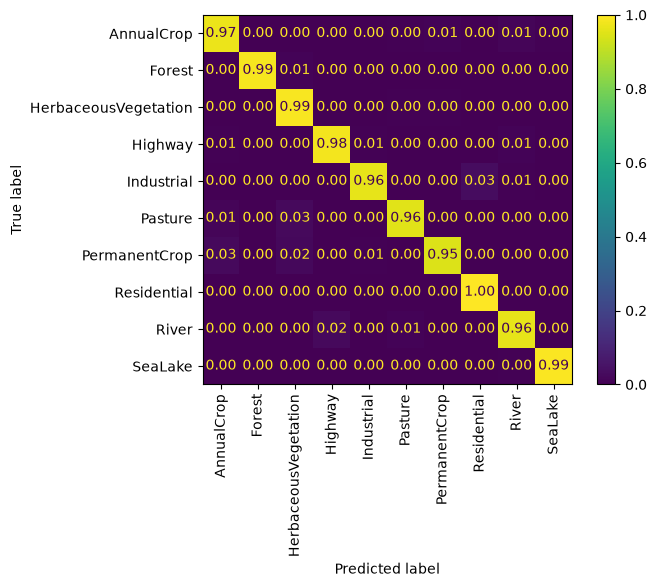
As we can see, the recall for residential plots was fantastic; all true residential images were accurately identified. Very few true Industrial images were incorrectly classified as residential.
Meanwhile, Permanent Crop was only correctly classified 95% of the time. Further work would involve investigating why.
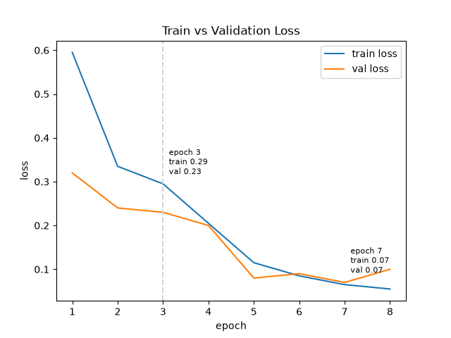
I do not see evidence here of overfitting; if the validation (orange) line rose while the training (blue) line stayed low, then I would be worried about overfitting.
What I do see is clear motivation and benefit of using the freeze and tune approach. The frozen model, at best, still had a loss of approximately 0.23. Once the model was unfrozen and allowed to fine tune, the loss dropped below 0.1.
Next Steps
Currently, this project only considers RGB and does not take advantage of all the bands that Sentinel-2 has to offer. I would like to further improve the model by considering all 13 bands, rather than staying limited to 3.
Code
Project Layout
eurosat/
├── README.md
├── .gitignore
├── src/
│   ├── data_preparation.py       split + transforms + dataloaders
│   └── evaluate.py               produce evaluation artifacts
├── notebooks/
│   ├── exploratory_data_analysis.ipynb      EDA workshop
│   └── learning_notes.ipynb                 notes from the process + questions
├── portfolio.ipynb   document used for my portfolio
└── data/             gitignored
AI Use
Claude was used in this project to help answer questions, organize my thoughts, and write my todo list so that I could focus on my learning goals. Claude was not used to write any training code. Claude did help with building the final plots so that I could focus on interpretation rather than visualization.
I prioritized understanding the implementation of a transfer learning approach over wrangling new syntax. I took notes as I learned, and used Claude to verify my notes for accuracy, for example:
Prompt:
are my notes accurate

#### What happens within an epoch

1. Forward pass
    * compute logits
    * pytorch records every operation performed on tensors
1. Compute Loss
1. Backward pass
    * Computes gradient of the loss wrt every trainable weight in the network
    * i.e. if you change one weight, how much does weight change and in what direction
    * graph in reverse (wrt forward pass)
    * computes chain rule at each step to determine how much each weight contributed the final loss value (is there more to the story here?)
    * results stored in weight.grad attribute
    * `backward()` does not update the weights, just computes and stores gradients
1. Update
    * `optimizer.step()` to record the ??
    * only updates the final layer (the 10 strata we care about)
AI Response:
Mostly accurate, a few corrections:

Forward pass: "records every operation performed on tensors" — more precisely, it records operations on tensors with requires_grad=True. That's the detail that explains why the frozen backbone doesn't show up in the backward pass at all — not because it's ignored afterward, but because no graph gets built for it in the first place.

Backward pass: "how much does weight change and in what direction" is off — a gradient isn't about how much the weight itself changes. It should read: if you change one weight slightly, how much does the loss change, and in what direction. That's what a gradient measures — sensitivity of the loss to that weight, not the weight to itself.

You asked "is there more to the story" on the chain-rule step — yes, one thing: gradients accumulate by default. If you call .backward() multiple times without clearing .grad in between, the new gradients add onto the old ones rather than replacing them. That's why training loops typically call optimizer.zero_grad() before each batch's backward pass — not part of backward() itself, but a required step around it that your notes don't have yet.

Update: "optimizer.step() to record the ??" — it doesn't record anything; it applies the update. It reads each parameter's .grad (computed by backward()) and adjusts the parameter's actual value using it (roughly, weight -= learning_rate * weight.grad, though the exact rule depends on the optimizer). This is the step where weights actually change — backward() only computed the gradients.

Also: "only updates the final layer" is true right now, specifically because the backbone is frozen — it's not a general fact about optimizer.step(). Once you unfreeze in the second phase, the same optimizer.step() call would update the whole network, assuming the optimizer is told about those newly-unfrozen parameters.
Sources
Footnotes
Eurosat: A novel dataset and deep learning benchmark for land use and land cover classification. Patrick Helber, Benjamin Bischke, Andreas Dengel, Damian Borth. IEEE Journal of Selected Topics in Applied Earth Observations and Remote Sensing, 2019.↩︎
Introducing EuroSAT: A Novel Dataset and Deep Learning Benchmark for Land Use and Land Cover Classification. Patrick Helber, Benjamin Bischke, Andreas Dengel. 2018 IEEE International Geoscience and Remote Sensing Symposium, 2018.↩︎
https://docs.pytorch.org/tutorials/beginner/transfer_learning_tutorial.html↩︎